bnSEM
bnSEM.RdbnSEM (Bayesian network SEM) translates OpenMx models to Bayesian networks fitted with bnlearn. The resulting network can be used to investigate conditional distributions of the SEM.
Value
list with
bayes_net: A fitted Bayesian network of class bn.fit
dag: The underlying directed acyclical graph
internal: Internal elements
Details
In Bayesian networks, all dependencies between variables must be expressed with directed "effects". There is no covariance in the same sense as in OpenMx. Instead, we must replace covariances with effects of a latent phantom variable. For instance x1 <-> x2 is replaced with ph -> y1; ph -> y2; ph <-> ph. The resulting model is identical to the initial OpenMx model in terms of fit, but the residual variance estimates will change.
bnSEM currently supports three different approaches:
First, when using phantom_type = "refit-free-loadings", bnSEM will add phantom variables only for covariances and re-estimate the SEM. For "refit-free-loadings", the loadings of the phantom on the observed variables is (1) constraint to equality if the covariance is positive and (2) constraint to have equal values, but opposite signs for covariances that are negative. The variance is constraint to one. This is based on a discussion with Prof. Marcel Paulssen for a bifactor modeling approach.
Second, when using phantom_type = "refit-free-single-loading", bnSEM will also add phantom variables only for covariances and re-estimate the SEM. However, in contrast to "refit-free-loadings" only one of the loadings is estimated, while the other one is constraint. This results in exactly the same fit as the first approach and is based on a suggestion by Dr. Christian Gische.
The advantage of the refitting approaches is that each manifest and latent variable of the original model will still have a residual variance in the new model and the Bayesian Network. This is necessary for cpdist to work as expected. The main disadvantages are that (1) refitting may fail and (2) constraints on the variance and covariance parameters cannot be accounted for.
Third, when using phantom_type = "cholesky", bnSEM will replace the full residual (co-)variance matrix with a Cholesky decomposition (S = DD^t). The latent and manifest variables (v) of the original model are now given by v = Du, where u is a vector of the same size as v with standard-normally distributed items. The main advantage of the Cholesky decomposition approach is that it does not require refitting the model and therefore also does not result in non-convergence. The main disadvantage is that each variable in the original model is now determined fully by the new variables in u. That is, none of the original variables has any residual variances in the new model. This can result in unexpected behavior when using cpdist on the model, where distributions for deterministic variables do not work. This approach has been suggested by Prof. Manuel C. Voelkle.
Examples
library(mxsem)
library(bnSEM)
model <- '
# latent variable definitions
ind60 =~ x1 + x2 + x3
dem60 =~ y1 + a*y2 + b*y3 + c*y4
dem65 =~ y5 + a*y6 + b*y7 + c*y8
# regressions
dem60 ~ ind60
dem65 ~ ind60 + dem60
# residual correlations
y1 ~~ y5
y2 ~~ y4 + y6
y3 ~~ y7
y4 ~~ y8
y6 ~~ y8
'
mx_model <- mxsem(model,
data = OpenMx::Bollen) |>
mxTryHard()
#> Running untitled1 with 39 parameters
#>
#> Beginning initial fit attempt
#> Running untitled1 with 39 parameters
#>
#> Lowest minimum so far: 3097.63615806793
#>
#> Solution found
#>
#>
#> Solution found! Final fit=3097.6362 (started at 226053.29) (1 attempt(s): 1 valid, 0 errors)
#> Start values from best fit:
#> 2.17965513767744,1.81820803128305,1.47132948979119,0.600476540990241,1.1907830045845,1.17453864934745,1.25097983167682,0.865040832989999,1.85464771778611,7.58135180193736,4.95567079105066,1.44012422593389,3.22448957283764,2.18302146917665,4.96820064436596,0.0813876183223778,0.120428272111891,0.466660220904411,0.582542038763785,2.31304366907279,0.711582171022699,3.56004988572433,0.362807663044655,1.37178930226827,3.30770431361029,0.448599494057923,3.87533800811413,0.164458467644595,5.4646672167648,4.25644221031117,6.56310926859193,4.45253418439515,2.97807466150035,5.05438421714178,4.79219524957923,3.55769039024485,5.13625221821929,6.19626503017659,4.04339056724364
network <- bnSEM::bnSEM(mx_model = mx_model)
#> Found covariances in your model. The model will be translated to an equivalent model with phantom variables. The model with phantom variables will be returned in the internal list as 'internal_model'
#> Refitting the model with phantom variables. The fit will be the same, but the variances of the residuals will change.
#> Running untitled1 with 39 parameters
#>
#> Beginning initial fit attempt
#> Running untitled1 with 39 parameters
#>
#> Lowest minimum so far: 3132.07452887361
#> Not all eigenvalues of the Hessian are positive: 7409.07977951187, 1708.4921031214, 655.260875997403, 625.899104490029, 457.72142428188, 376.258200994535, 366.924619040786, 271.011429005247, 265.437567430202, 157.393760304802, 111.339097771214, 72.616612034957, 63.9297690322516, 61.0383050737711, 56.627072254474, 54.3105925229991, 45.2632627355016, 41.9346170781772, 39.9711018611112, 37.1099691494525, 27.9475214045914, 23.504335315514, 13.8159828264391, 13.4584620171711, 10.1163268846973, 5.93679347294567, 4.63952548317951, 4.24632667695603, 3.04163267507704, 2.68408652935071, 2.61509853800472, 2.13390599951173, 1.33725658409888, -7.89480847384507, -12.9932368828123, -14.4031732798695, -17.401512022946, -22.8381101841975, -36.5544156727883
#>
#> Beginning fit attempt 1 of at maximum 10 extra tries
#> Running untitled1 with 39 parameters
#>
#> Lowest minimum so far: 3132.0745288736
#> Not all eigenvalues of the Hessian are positive: 7409.07946631424, 1708.49176254252, 655.262286350761, 625.899786188011, 457.721685876745, 376.260783922478, 366.932528233966, 271.009859911427, 265.438524600836, 157.396807010254, 111.342585804438, 72.6167766533036, 63.9352311045493, 61.0390482740306, 56.6339623736013, 54.3104453763072, 45.2632686570807, 41.9351454711872, 39.9767382744959, 37.1099239340399, 27.946888841747, 23.5034088419334, 13.8164979122581, 13.4625242475388, 10.1176775901302, 5.93688486525776, 4.64105325462696, 4.24682194640139, 3.04155839709106, 2.68485416828844, 2.61522710656298, 2.1339753363589, 1.33755296918274, -7.89552985437282, -12.9932320995248, -14.39474901683, -17.3937882550772, -22.8219453788941, -36.554413874216
#>
#> Beginning fit attempt 2 of at maximum 10 extra tries
#> Running untitled1 with 39 parameters
#>
#> Lowest minimum so far: 3132.07452887354
#> Not all eigenvalues of the Hessian are positive: 7409.07755515461, 1708.49179450561, 655.269018739405, 625.904731956063, 457.721216593275, 376.266395763769, 366.940360898295, 271.016420528627, 265.445378915433, 157.403686520319, 111.344026810214, 72.6164364448542, 63.9411636309463, 61.0384141267404, 56.6459876508006, 54.3104338818113, 45.2630482445342, 41.9349710701663, 39.9777283916397, 37.1096191019541, 27.9471671029214, 23.503821576877, 13.8195204570364, 13.4656916133495, 10.1184430302727, 5.93788731343455, 4.6421197361214, 4.24805452974307, 3.04254921541662, 2.68559198738686, 2.61556886539968, 2.1343145244916, 1.33783463767334, -7.87939297174849, -12.9855013329785, -14.3863270812647, -17.3846851695095, -22.8219259369459, -36.5466883847122
#>
#> Beginning fit attempt 3 of at maximum 10 extra tries
#> Running untitled1 with 39 parameters
#>
#> Lowest minimum so far: 3097.6361580659
#>
#> Solution found
#>
#>
#> Solution found! Final fit=3097.6362 (started at 3134.3045) (4 attempt(s): 4 valid, 0 errors)
#> Start values from best fit:
#> 2.17965694601052,1.8182095011406,1.47133099598838,0.600474653668476,1.19078350357395,1.17454016540082,1.25098064748735,0.865041423996671,0.763246442204963,1.2000523657831,-1.47750116242389,-0.843553738394088,-0.602332059455713,-1.17123333497147,1.27210511655049,3.95820573640009,4.2440902031704,1.42155802177756,1.41339221020283,0.0813876987310841,0.120427701910668,0.466659891686399,1.73049836432522,2.8484543853871,1.57310358628673,0.448599049551262,3.87532058399932,0.164463388633157,5.46466667088102,4.25644287857883,6.56311025543758,4.45253304354606,2.97807408933287,5.05438384047728,4.79219462734189,3.55768978686791,5.13625192503549,6.19626389645749,4.04338968668393
# plot network
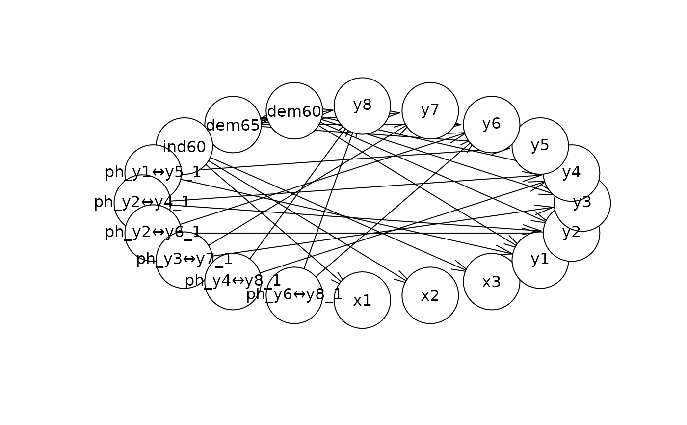
plot(network$dag)
 # Check conditional distribution
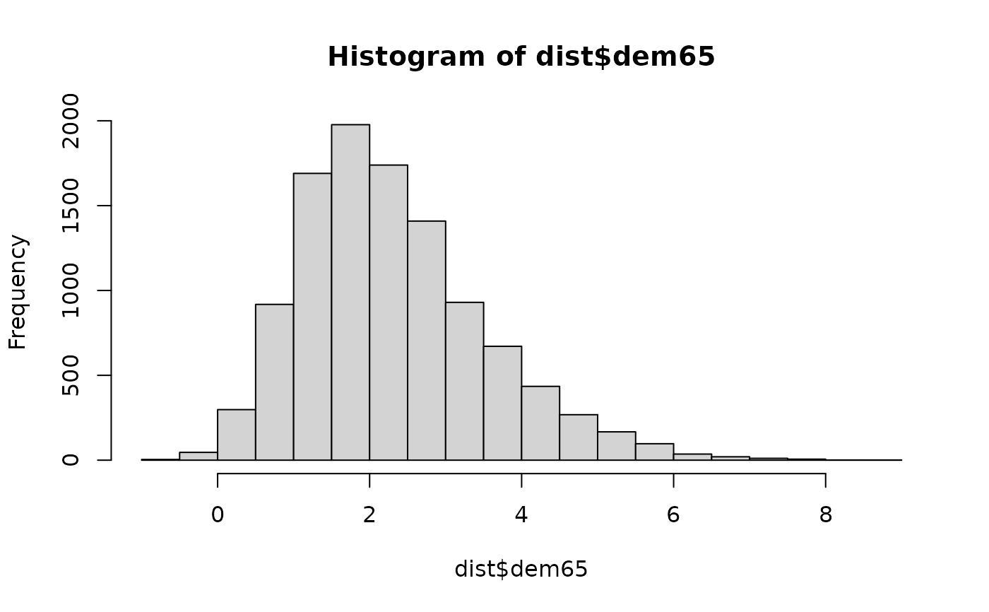
# probability that dem65 in (1,2) given dem60 > 1:
bnlearn::cpquery(fitted = network$bayes_net,
event = (dem65 > 1 & dem65 < 2),
evidence = (dem60 > 1))
#> [1] 0.3447854
# Get distribution under this assumption:
dist <- bnlearn::cpdist(fitted = network$bayes_net,
node = "dem65",
evidence = (dem60 > 1))
hist(dist$dem65)
# Check conditional distribution
# probability that dem65 in (1,2) given dem60 > 1:
bnlearn::cpquery(fitted = network$bayes_net,
event = (dem65 > 1 & dem65 < 2),
evidence = (dem60 > 1))
#> [1] 0.3447854
# Get distribution under this assumption:
dist <- bnlearn::cpdist(fitted = network$bayes_net,
node = "dem65",
evidence = (dem60 > 1))
hist(dist$dem65)
 # simulate data from the network and refit SEM to check if the estimates align:
sim <- bnlearn::rbn(x = network$bayes_net, n = 10000)
fit_sim <- mxsem(model,
data = sim[,mx_model$manifestVars]) |>
mxTryHard()
#> Running untitled38 with 39 parameters
#>
#> Beginning initial fit attempt
#> Running untitled38 with 39 parameters
#>
#> Lowest minimum so far: 17703119.5195107
#> OpenMx status code 6 not in list of acceptable status codes, (0,0)
#> Not all eigenvalues of the Hessian are positive: 2914338498.44273, 1812869865.95158, 1084954935.5846, 297212090.027587, 291973388.879885, 201545721.511776, 77711373.4250763, 61338573.7212463, 56078869.5418081, 44082464.1203594, 29475786.810217, 17210094.8330976, 12114265.3559555, 5658244.07604814, 5027522.97244289, 2885840.43479572, 1793254.59081873, 1432868.6585753, 1306320.30170179, 1132950.09688801, 918391.257137507, 643675.24184825, 401318.847882216, 328886.524197269, 288667.321154138, 147691.516446736, 66960.0131415541, 45316.5536944429, 44803.7782716291, 28827.7038644157, 16521.9760572714, 13522.2250711224, 9877.5459626002, 8999.90928061198, 5431.86868581075, 3911.40645385117, -713725.72758759, -18463926.4595984, -33723510.4312441
#>
#> Beginning fit attempt 1 of at maximum 10 extra tries
#> Running untitled38 with 39 parameters
#>
#> Lowest minimum so far: 413369.288632004
#>
#> Solution found
#>
#>
#> Solution found! Final fit=413369.29 (started at 29964553) (2 attempt(s): 2 valid, 0 errors)
#> Start values from best fit:
#> 2.16627427525228,1.7984159157888,1.46360461006967,0.612532022592901,1.19051519797498,1.183071028878,1.25339515280699,0.863522916008263,1.87001685447078,7.55509984343051,5.00113309825581,1.41850312719469,3.24628072102026,2.14786252370429,4.85642827145101,0.0801346348576689,0.133036608810701,0.452910665114826,0.638811377158028,2.417420535993,0.658467110230315,3.54523898226212,0.330828491210027,1.29270006753386,3.23219579001001,0.459682466016011,3.81854049877937,0.171211877754727,5.45174115463114,4.23699910113603,6.54812202910106,4.47180930709653,2.94698953612172,5.05064003805534,4.78367017508737,3.5616462187411,5.11127646830139,6.14553461128183,4.0317302839105
round(abs(coef(fit_sim) -
coef(mx_model)) / abs(coef(mx_model)), 3)
#> ind60→x2 ind60→x3 ind60→dem60 ind60→dem65 a b
#> 0.006 0.011 0.005 0.020 0.000 0.007
#> c dem60→dem65 y1↔y1 y2↔y2 y3↔y3 y2↔y4
#> 0.002 0.002 0.008 0.003 0.009 0.015
#> y4↔y4 y2↔y6 y6↔y6 x1↔x1 x2↔x2 x3↔x3
#> 0.007 0.016 0.022 0.015 0.105 0.029
#> y1↔y5 y5↔y5 y3↔y7 y7↔y7 y4↔y8 y6↔y8
#> 0.097 0.045 0.075 0.004 0.088 0.058
#> y8↔y8 ind60↔ind60 dem60↔dem60 dem65↔dem65 one→y1 one→y2
#> 0.023 0.025 0.015 0.041 0.002 0.005
#> one→y3 one→y4 one→y6 one→x1 one→x2 one→x3
#> 0.002 0.004 0.010 0.001 0.002 0.001
#> one→y5 one→y7 one→y8
#> 0.005 0.008 0.003
# simulate data from the network and refit SEM to check if the estimates align:
sim <- bnlearn::rbn(x = network$bayes_net, n = 10000)
fit_sim <- mxsem(model,
data = sim[,mx_model$manifestVars]) |>
mxTryHard()
#> Running untitled38 with 39 parameters
#>
#> Beginning initial fit attempt
#> Running untitled38 with 39 parameters
#>
#> Lowest minimum so far: 17703119.5195107
#> OpenMx status code 6 not in list of acceptable status codes, (0,0)
#> Not all eigenvalues of the Hessian are positive: 2914338498.44273, 1812869865.95158, 1084954935.5846, 297212090.027587, 291973388.879885, 201545721.511776, 77711373.4250763, 61338573.7212463, 56078869.5418081, 44082464.1203594, 29475786.810217, 17210094.8330976, 12114265.3559555, 5658244.07604814, 5027522.97244289, 2885840.43479572, 1793254.59081873, 1432868.6585753, 1306320.30170179, 1132950.09688801, 918391.257137507, 643675.24184825, 401318.847882216, 328886.524197269, 288667.321154138, 147691.516446736, 66960.0131415541, 45316.5536944429, 44803.7782716291, 28827.7038644157, 16521.9760572714, 13522.2250711224, 9877.5459626002, 8999.90928061198, 5431.86868581075, 3911.40645385117, -713725.72758759, -18463926.4595984, -33723510.4312441
#>
#> Beginning fit attempt 1 of at maximum 10 extra tries
#> Running untitled38 with 39 parameters
#>
#> Lowest minimum so far: 413369.288632004
#>
#> Solution found
#>
#>
#> Solution found! Final fit=413369.29 (started at 29964553) (2 attempt(s): 2 valid, 0 errors)
#> Start values from best fit:
#> 2.16627427525228,1.7984159157888,1.46360461006967,0.612532022592901,1.19051519797498,1.183071028878,1.25339515280699,0.863522916008263,1.87001685447078,7.55509984343051,5.00113309825581,1.41850312719469,3.24628072102026,2.14786252370429,4.85642827145101,0.0801346348576689,0.133036608810701,0.452910665114826,0.638811377158028,2.417420535993,0.658467110230315,3.54523898226212,0.330828491210027,1.29270006753386,3.23219579001001,0.459682466016011,3.81854049877937,0.171211877754727,5.45174115463114,4.23699910113603,6.54812202910106,4.47180930709653,2.94698953612172,5.05064003805534,4.78367017508737,3.5616462187411,5.11127646830139,6.14553461128183,4.0317302839105
round(abs(coef(fit_sim) -
coef(mx_model)) / abs(coef(mx_model)), 3)
#> ind60→x2 ind60→x3 ind60→dem60 ind60→dem65 a b
#> 0.006 0.011 0.005 0.020 0.000 0.007
#> c dem60→dem65 y1↔y1 y2↔y2 y3↔y3 y2↔y4
#> 0.002 0.002 0.008 0.003 0.009 0.015
#> y4↔y4 y2↔y6 y6↔y6 x1↔x1 x2↔x2 x3↔x3
#> 0.007 0.016 0.022 0.015 0.105 0.029
#> y1↔y5 y5↔y5 y3↔y7 y7↔y7 y4↔y8 y6↔y8
#> 0.097 0.045 0.075 0.004 0.088 0.058
#> y8↔y8 ind60↔ind60 dem60↔dem60 dem65↔dem65 one→y1 one→y2
#> 0.023 0.025 0.015 0.041 0.002 0.005
#> one→y3 one→y4 one→y6 one→x1 one→x2 one→x3
#> 0.002 0.004 0.010 0.001 0.002 0.001
#> one→y5 one→y7 one→y8
#> 0.005 0.008 0.003